Empty Pipes
Slowing Down the Force Directed Graph in D3
Tracking the stepwise movements of the force-directed graph layout in d3.js is useful when creating more intricate and/or dynamic graphs. Unfortunately, in its current implementations, these changes are fleeting and hard to see due to the speed with which the layout is updated. Slowing it down can help to see how each tick event updates the positions of each node. A method for doing this is described by @DavidBruant in a thread about running the force simulation faster. Keep in mind that this is a hack and probably shouldn’t be used for anything production-related.
Implementing this slowdown requires slightly changing d3.js. To adjust the desired
delay between each tick event, simply change the setTimeout(tick, 234) line.
pkerp@toc:~/projects/emptypipes$ diff js/d3.js js/d3_slow.js
6228c6228,6233
<         d3.timer(force.tick);
---
>         setTimeout(function tick(){
>             force.tick();
>             if(alpha >= .005)
>                 setTimeout(tick, 234);
>         }, 0);
>         //d3.timer(force.tick);
The modified version of d3.js used in the ‘slow’ example abov used in the ‘slow’ example abovee is available here.
Selectable Force-Directed Graph Using D3.js
Update: An new version of this example using D3v4 can be found in a more recent blog post.
Dragging multiple nodes in a force-directed graph layout is useful for making large changes in its arrangement. Mike Bostock showed a nice example of this while describing the process of creating the 2013 Oscar Contenders visualization in his Eyeo talk about examples.
His example, while instructive and useful, can be made even more helpful by adding the dynamic force calculation, as well as zooming and centering behaviour.
In the example below, hold down shift to select multiple nodes or press the ‘c’ key to center the graph. Zooming and panning follow the typical pattern using the mousewheel and dragging.
The selection process is made to emulate the behaviour of selection and dragging that is seen in most file managers and is thus familiar to most users of desktop computers:
- Clicking on a node selects it and de-selects everything else.
- Shift-clicking on a node toggles its selection status and leaves all other nodes as they are.
- Shift-dragging toggles the selection status of all nodes within the selection area.
- Dragging on a selected node drags all selected nodes.
- Dragging an unselected node selects and drags it while de-selecting everything else.
Finally, the cursor is changed to a crosshair when the user presses the shift key.
The code for this example is available on bl.ocks.org or directly from github gist. An example of its use is found in this RNA secondary structure visualization tool.
Python vs. Scala vs. Spark
Update 20 Jan 2015
Thanks to a suggestion from a reddit comment, I added benchmarks for the python code running under PyPy. This makes the results even more interesting. PyPy actually runs the join faster than Scala when more cores are present. On the other hand, it runs the sort slower, leading to an approximately equal performance when there are more than 2 cores available. This is really good news for people (like myself) who are more familiar with python and don’t want to learn another language just to execute faster Spark queries.
Apart from the extra data in the charts, the rest of this post is unmodified and thus doesn’t mention PyPy.
The fantastic Apache Spark framework provides an API for distributed data analysis and processing in three different languages: Scala, Java and Python. Being an ardent yet somewhat impatient Python user, I was curious if there would be a large advantage in using Scala to code my data processing tasks, so I created a small benchmark data processing script using Python, Scala, and SparkSQL.
The Task
The benchmark task consists of the following steps:
- Load a tab-separated table (gene2pubmed), and convert string values to integers (map, filter)
- Load another table (pmid_year), parse dates and convert to integers (map)
- Join the two tables on a key (join)
- Rearrange the keys and values (map)
- Count the number of occurances of a key (reduceByKey)
- Rearrange the keys and values (map)
- Sort by key (sortByKey)
The Data
The dataset consists of two text file tables, weighing in at 297M and 229M.
Total Running Time
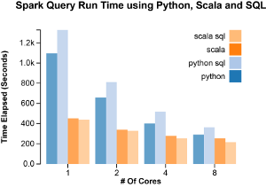
Each of the scripts was run with a collect statement at the end to ensure that
each step was executed. The time was recorded as the real time elapsed between
the start of the script and the end. The scripts were run using 1,2,4 and 8
worker cores (as set by the SPARK_WORKER_CORES option).
The fastest performance was achieved when using SparkSQL with Scala. The slowest, SparkSQL with Python. The more cores used, the more equal the results. This is likely due to the fact that parallelizable tasks start to contribute less and less of the total time and so the running time becomes dominated by the collection and aggregation which must be run synchronously, take a long time and are largely language independent (i.e. possibly run by some internal Spark API).
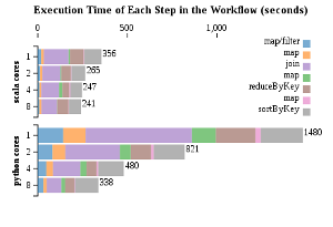
To get a clearer picture of where the differences in performance lie, a count()
action was performed after each transformation and other action. The time was
recorded after each count().
This data indicates that just about every step in the Python implementation, except for the final sort, benefitted proportionally (~ 8x) from the extra cores. The Scala implementation, in contrast, showed no large speedup in any of the steps. The longest, the join and sort steps, ran about 1.5 times faster when using 8 cores vs when using just 1. This can be either because the dataset is too small to benefit from parallelization, given Scala’s already fast execution, or that something strange is going on with the settings and the operations performed by the master node are being run concurrently even when there are less worker nodes available.
This doesn’t appear to be case as running both the master and worker nodes on a machine with only four available cores (vs 24 in the previous benchmarks) and allowing only one worker core actually led to faster execution. A more comprehensive test would require running the master node on a single core machine and placing the workers on separate more capable computers. I’ll save that for another day though.
Conclusion
If you have less cores at your disposal, Scala is quite a bit faster than Python. As more cores are added, its advantage dwindles. Having more computing power gives you the opportunity to use alternative languages without having to wait for your results. If computing resources are at a premium, then it might make sense to learn a little bit of Scala, if only enough to be able to code SparkSQL queries.
Apache Spark
The code for each programming language is listed in the sections below:
Master and Worker Nodes
The number of workers was set in the SPARK_WORKER_CORES variable in conf/spark-env.sh
./sbin/stop-all.sh; rm logs/*; ./sbin/start-all.shPython Shell
./spark-1.2.0/bin/pyspark --master spark://server.com:7077 --driver-memory 4g --executor-memory 4gScala Shell
./spark-1.2.0/bin/spark-shell --master spark://server.com:7077 --driver-memory 4g --executor-memory 4gBenchmark Code
The following code was pasted into its respective shell and timed.
Scala
val pmid_gene = sc.textFile("/Users/pkerp/projects/genbank/data/gene2pubmed").map(_.split("\t")).filter(_(0).head != '#').map(line => (line(2).toInt, line(1).toInt)).cache()

// the dates were obtained by doing entrez queries and stored as
// table of the form "date pmid"
	object ParsingFunctions {
		def parseDate(line: String): (Int,Int) = {
		    // extract the date information and the pmid
		    // and return it as tuple
		    val parts = line.split(" ");
			// the year is in %Y/%m/%d format
			val year = parts(0).split("/")(0).toInt;
			val pmid = parts(1).toInt;
			return (pmid, year);
		}
	}
val pmid_year = sc.textFile("/Users/pkerp/projects/genbank/data/pmid_year.ssv").map(ParsingFunctions.parseDate)
val pmid_gene_year = pmid_year.join(pmid_gene)

val gene_year_1 = pmid_gene_year.map{ case (pmid, (gene, year)) => ((gene, year), 1)}
val gene_year_counts = gene_year_1.reduceByKey((x,y) => x+y)
val counts_gene_year = gene_year_counts.map{case ((gene,year), count) => (count, (gene, year))}
val sorted_counts_gene_year = counts_gene_year.sortByKey()
val scgy = sorted_counts_gene_year.collect()
//blah
Scala SQL
val sqlContext = new org.apache.spark.sql.SQLContext(sc)
import sqlContext.createSchemaRDD
case class PmidGene(taxid: Int, geneid: Int, pmid: Int)
case class PmidYear(pmid: Int, year: Int)

val gene2pubmed = sc.textFile("/Users/pkerp/projects/genbank/data/gene2pubmed").map(_.split("\t")).filter(_(0).head != '#').map(line => PmidGene(line(0).toInt, line(1).toInt, line(2).toInt)).cache()

gene2pubmed.registerTempTable("gene2pubmed")

	object ParsingFunctions {
		def parseDate(line: String): PmidYear = {
		    // extract the date information and the pmid
		    // and return it as tuple
		    val parts = line.split(" ");
			// the year is in %Y/%m/%d format
			val year = parts(0).split("/")(0).toInt;
			val pmid = parts(1).toInt;

			return PmidYear(pmid, year);
		}
	}

val pmid_year = sc.textFile("/Users/pkerp/projects/genbank/data/pmid_year.ssv").map(ParsingFunctions.parseDate)
pmid_year.registerTempTable("pmid_year")
val geneid_year = sqlContext.sql("select geneid, year from pmid_year, gene2pubmed where pmid_year.pmid = gene2pubmed.pmid")
geneid_year.registerTempTable("geneid_year")
val result = sqlContext.sql("select geneid, year, count(*) as cnt from geneid_year group by geneid, year order by cnt desc")
val x = result.collect()
//blah
Python
# get the gene_id -> pubmed mapping
pmid_gene = sc.textFile("/Users/pkerp/projects/genbank/data/gene2pubmed").map(lambda x: x.split("\t")).filter(lambda x: x[0][0] != '#').map(lambda x: (int(x[2]), int(x[1]))).cache()

# the dates were obtained by doing entrez queries and stored as
# table of the form "date pmid"
def parse_date_pmid_line(line):
    # extract the date information and the pmid
    # and return it as tuple
    parts = line.split()
    # the year is in %Y/%m/%d format
    year = int(parts[0].split('/')[0])
    pmid = int(parts[1])
    return (pmid, year)

# extract the dates and store them as values where the key is the pmid
pmid_year = sc.textFile('/Users/pkerp/projects/genbank/data/pmid_year.ssv').map(parse_date_pmid_line).cache()
pmid_gene_year = pmid_year.join(pmid_gene)

gene_year_1 = pmid_gene_year.map(lambda (pmid, (gene, year)): ((gene,year),1))
gene_year_counts = gene_year_1.reduceByKey(lambda x,y: x+y)
counts_gene_year = gene_year_counts.map(lambda ((gene, year), count): (count, (gene, year)))
sorted_counts_gene_year = counts_gene_year.sortByKey(ascending=False);
scgy = sorted_counts_gene_year.collect()
#blah
Python SQL
from pyspark.sql import *
sqlContext = SQLContext(sc)
# get the gene_id -> pubmed mapping
gene2pubmed = sc.textFile("/Users/pkerp/projects/genbank/data/gene2pubmed").filter(lambda x: x[0] != '#').map(lambda x: x.split('\t')).map(lambda p: Row(taxid=int(p[0]), geneid=int(p[1]), pmid=int(p[2])))
schemaGene2Pubmed = sqlContext.inferSchema(gene2pubmed)
schemaGene2Pubmed.registerTempTable("gene2pubmed")
# the dates were obtained by doing entrez queries and stored as
# table of the form "date pmid"
def parse_date_pmid_line(line):
    # extract the date information and the pmid
    # and return it as tuple
    parts = line.split()
    # the year is in %Y/%m/%d format
    year = int(parts[0].split('/')[0])
    pmid = int(parts[1])
    return (pmid, year)


pmid_year = sc.textFile('/Users/pkerp/projects/genbank/data/pmid_year.ssv').map(parse_date_pmid_line).map(lambda p: Row(pmid=p[0], year=p[1]))
schemaPmidYear = sqlContext.inferSchema(pmid_year)
schemaPmidYear.registerTempTable('pmid_year')
geneid_year = sqlContext.sql('select geneid, year from pmid_year, gene2pubmed where pmid_year.pmid = gene2pubmed.pmid')
geneid_year.registerTempTable('geneid_year')
result = sqlContext.sql('select geneid, year, count(*) as cnt from geneid_year group by geneid, year order by cnt desc')
x = result.collect()
#blah
